Category Archives: EDS

Good Companies, Troubled Stocks and Potential Opportunity

Truth be told I am not much of a “stock picker”. Oh, I can pick ‘em alright just like anyone else.  They just to don’t go the right way as often as I’d like.  I also believe that the way to maximize profitability is to follow a momentum type approach that identifies stocks that are performing well and buying them when they breakout to the upside (ala O’Neil, Minervini, Zanger, etc.) and then riding them as long as they continue to perform.  Unfortunately, I’m just not very good at it. 

Back when I started out, there was such a thing as a “long-term investor.”  People would try to find good companies selling at a decent price and they would buy them and hold them for, well, the long-term.  Crazy talk, right? As I have already stated, I am not claiming that that is a better approach. I am just pointing out that it was “a thing.”

An Indicator

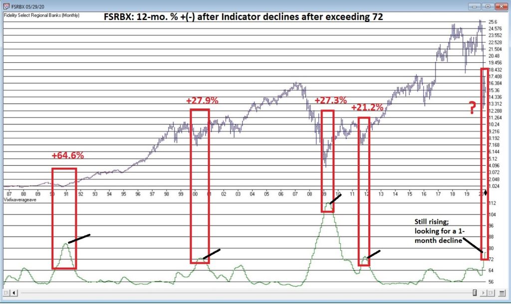
There is an indicator (I will call it VFAA, which is short for vixfixaverageave, which – lets face it – is a terrible name) that I follow that was developed as an extension of Larry William’s VixFix Indicator.  There is nothing magic about it.  Its purpose is to identify when price has reached an exceptionally oversold level and “may” be due to rally.  The code for this indicator appears later.

For the record, I DO NOT systematically use this indicator in the manner I am about to describe, nor am I recommending that you do.  Still, it seems to have some potential value, so what follows is merely an illustration for informational purposes only.

The Rules

*We will look at a monthly bar chart for a given stock

*A “buy signal” occurs when VFAA reaches or exceeds 80 and then turns down for one month

*A “sell (or exit) signal” occurs when VFAA subsequently rises by at least 0.25 from a monthly closing low

Seeing as how this is based solely on monthly closes it obviously this is not going to be a “precision market timing tool.”

Some “Good Companies” with “Troubled Stocks”

So now let’s apply this VFAA indicator to some actual stocks.  Again, I AM NOT recommending that anyone use this approach mechanically.  The real goal is merely to try to identify situations where a stock has been washed out, reversed and MAY be ready to run for a while.

Ticker BA

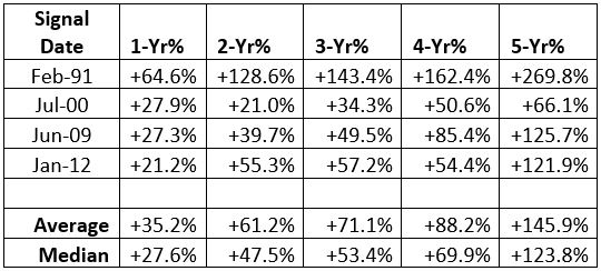
Figure 1 displays a monthly chart for Boeing (BA) with VFAA at the bottom.  The numbers on the chart represent the hypothetical + (-) % achieved by applying the rules above (although once again, to be clear I am not necessarily suggesting anyone use it exactly this way). 

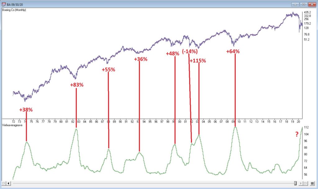
Figure 1 – Ticker BA with VFAA (Courtesy AIQ TradingExpert)

From March 2019 into March 2020 BA declined -80%.  It has since bounced around and VFAA has soared to 110.88.  VFAA has yet to rollover on a month-end basis, so nothing to do here except exhibit – what’s that word again – oh right, “patience.”

Ticker GD

Figure 2 displays a monthly chart for General Dynamics (GD) with VFAA at the bottom. 

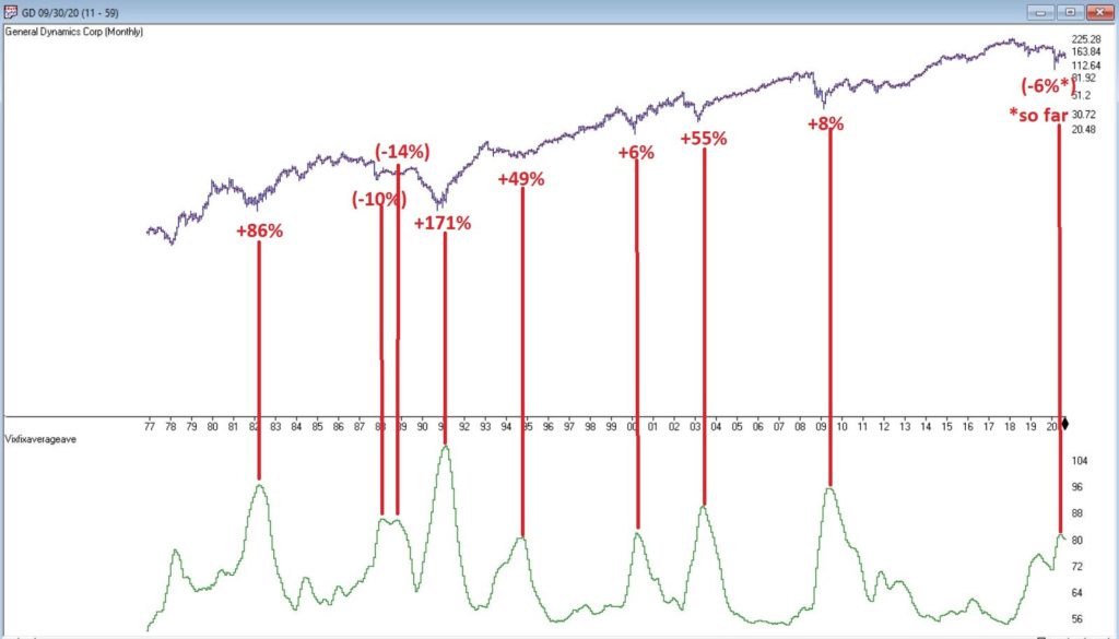
Figure 2 – Ticker GD with VFAA (Courtesy AIQ TradingExpert)

Are these “world-beating numbers”?  Not really.  But in terms of helping to identify potential opportunities, not so bad. VFAA gave a “buy signal” for GD at the end of July. So far, not so good as the stock is down about -6%.

Ticker WFC

Figure 3 displays a monthly chart for Wells Fargo (WFC) with VFAA at the bottom. 

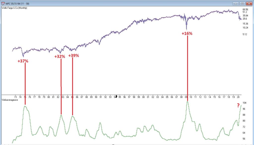
Figure 3 – Ticker WFC with VFAA (Courtesy AIQ TradingExpert)

There are not many “signals” but the ones that occurred have been useful. Between 2018 and 2020 WFC declined -65%.  It has since bounced around and VFAA has soared to 102.44.  VFAA has yet to rollover on a month-end basis. But at some point it will, and a potential opportunity may arise.

VFAA Formula

Below is the code for VFAA

VixFix is an indicator developed many years ago by Larry Williams which essentially compares the latest low to the highest close in the latest 22 periods (then divides the difference by the highest close in the latest 22 periods).  I then multiply this result by 100 and add 50 to get VixFix.

*Next is a 3-period exponential average of VixFix

*Then VFAA is arrived at by calculating a 7-period exponential average of the previous result (essentially, we are “double-smoothing” VixFix)

Are we having fun yet?  See code below:

hivalclose is hival([close],22).

vixfix is (((hivalclose-[low])/hivalclose)*100)+50.

vixfixaverage is Expavg(vixfix,3).

vixfixaverageave is Expavg(vixfixaverage,7).

VFAA = vixfixaverageave

EDITORS NOTE: The AIQ Expert Design Studio code for the indicator is available to download from here. Save this file to your /wintes32/EDS Strategies folder https://aiqeducation.com/VFAA.EDS

Summary

One thing to note is that VFAA “signals” on a monthly chart don’t come around very often.  So, you can’t really sit around and wait for a signal to form on your “favorite company”.  You have to look for opportunity wherever it might exist.

One last time let me reiterate that I am not suggesting using VFAA as a standalone systematic approach to investing. But when a signal does occur – especially when applied to quality companies that have recently been “whacked”, it can help to identify a potential opportunity.

Jay Kaeppel

Disclaimer: The information, opinions and ideas expressed herein are for informational and educational purposes only and are based on research conducted and presented solely by the author.  The information presented represents the views of the author only and does not constitute a complete description of any investment service.  In addition, nothing presented herein should be construed as investment advice, as an advertisement or offering of investment advisory services, or as an offer to sell or a solicitation to buy any security.  The data presented herein were obtained from various third-party sources.  While the data is believed to be reliable, no representation is made as to, and no responsibility, warranty or liability is accepted for the accuracy or completeness of such information.  International investments are subject to additional risks such as currency fluctuations, political instability and the potential for illiquid markets.  Past performance is no guarantee of future results.  There is risk of loss in all trading.  Back tested performance does not represent actual performance and should not be interpreted as an indication of such performance.  Also, back tested performance results have certain inherent limitations and differs from actual performance because it is achieved with the benefit of hindsight.

Vitali Apirine’s – The Compare Price Momentum Oscillator (CPMO)

The importable AIQ EDS file based on Vitali Apirine’s article in the August, 2020 issue of Stocks & Commodities magazine, “The Compare Price Momentum Oscillator (CPMO),” can be obtained on request via email to info@TradersEdgeSystems.com.

… Here is a way you can compare at a glance the momentum of two different market indexes or securities in the same chart. It could also be used to help generate trading signals. In this first part of a three-part series, we’ll look at comparing index momentums…

The code is also available here:

!Author: Vitali Aprine, TASC August 2020
!Coded by: Richard Denning, 6/20/20
!www.TradersEdgeSystems.com

!Custom smoothing multiplier: 2 / time period
!PMO line: 20-period custom EMA of (10 × 35-period
!custom EMA of ((Today’s price – Yesterday’s price) / !Yesterday’s price × 100))
!PMO signal line: 10-period EMA of the PMO line

Len1 is 20.
Len2 is 35.
Len3 is 10.
Ticker1 is “QQQ”.
Ticker2 is “SPY”.

C is [close].
C1 is valresult(C,1).
RC1 is (C/C1*100)-100.

custSmoLen1 is Len1 – 1.
custSmoLen2 is Len2 – 1.

CustEma is 10*expavg(RC1,custSmoLen2).
PMO is expavg(CustEma,custSmoLen1).
PMOsig is expavg(PMO,Len3).

Ticker1C is tickerUDF(Ticker1,C).
RC1ticker1 is (Ticker1C/valresult(Ticker1C,1)*100)-100.
CustEmaTicker1 is 10*expavg(RC1ticker1,custSmoLen2).
PMOticker1 is expavg(CustEmaTicker1,custSmoLen1).

Ticker2C is tickerUDF(Ticker2,C).
RC1ticker2 is (Ticker2C/valresult(Ticker2C,1)*100)-100.
CustEmaTicker2 is 10*expavg(RC1ticker2,custSmoLen2).
PMOticker2 is expavg(CustEmaTicker2,custSmoLen1).

CPMO is PMOTicker1 – PMOTicker2.
List if hasdatafor(1000) >= 900.

I coded the indicator described by the author. Figure 10 shows the indicator (QQQ,SPY,20,35) on chart of IWM. When the white line is above the red line on the CPMO indicator, this indicates that the QQQ is stronger than the SPY. Generally, it is considered bullish when the QQQ is leading in strength.

Sample Chart

FIGURE 10: AIQ. The CPMO indicator is shown on a chart of IWM with parameters (QQQ,SPY,20,35).

—Richard Denning
info@TradersEdgeSystems.com
for AIQ Systems

Financials – Danger or Opportunity? Or Both?

To say that there is has been and remains a great deal of angst in the financial markets is a bit of an understatement. This is especially true when it comes to the financial sector.  The financial sector has a fairly high correlation to treasury yields (ticker FSRBX – Fidelity Select Banking Portfolio has a 0.52 correlation to ticker TNX – which tracks 10-year treasury yields).  As yields have plummeted so has the financial sector.  During the recent decline, FSRBX plunged -51% from its December 2019 peak.  With little expectation of higher rates anytime soon a lot of investors are understandably wary of diving into this sector.

But much like with the energy sector, the old adage that the time to buy is when there is “blood in the streets”, should give one pause before they turn their back completely on the financial sector.  For the time being I am keeping my eye on a little-known indicator called “Vixfixaverageave” (yes, I agree it is a really bad name).  The calculations for this indicator appear at the end of this article.  The reason I am watching it right now is that it recently reached a very oversold level that has helped to highlight some useful buying opportunities for financials in the past.

Ticker FSRBX

Figure 1 displays a monthly chart for FSRBX in the top clip and the Vixfixaverageave indicator in the bottom clip.  Note that the indicator rose above 72 at the end of April 2020.  As you can see there have been four previous occasions when this indicator, a) exceeded 72 and then b) reversed lower for one month.  For arguments sake we will call that a buy signal.

Figure 1 – Ticker FSRBX with indicator Vixfixaverageave (Courtesy AIQ TradingExpert)

Figure 2 displays the 1 to 5 year % + (-) for FSRBX following the four previous signals.  As you can see, they all proved to be exceptional buying opportunities.

Figure 2 – FSRBX returns 1 to 5 years after signal

Now for the disappointing news: if you are thinking that all we have to do is wait for this indicator to finally top out and that big profits are “guaranteed” to roll in, you are making a mistake.  As they say, “past performance is no guarantee of future results.”  (Sorry, I don’t make the rules).  So, when the Vixfixaverageave monthly reading for FSRBX does finally roll over, the proper course of action would be to:

*Decide if you really want to act based on the signal

*Decide how much capital you are willing to commit

*Decide how much of that capital you are actually willing to risk – i.e. will you stop out if a loss exceeds x%, or do you plan to simply hold it for 1 to 5 years regardless?

Summary

There are a million and one ways to trigger an entry signal.  The one discussed herein is just one more.  What really separates the winners from the losers is the answers to the three questions just posed.

Vixfixaverageave Calculations 

EDITTORS NOTE: The code sections can be copied and pasted into AIQ EDS or you can download the indicator code in an EDS file from here and save it to your /wintes32/EDS Strategies folder.

This indicator is based on another indicator called VixFix which was developed many years ago by Larry Williams.

hivalclose is hival([close],22).  <<<<<The high closing price in that last 22 periods

vixfix is (((hivalclose-[low])/hivalclose)*100)+50. <<<(highest closing price in last 22 periods minus current period low) divided by highest closing price in last 22 periods (then multiplied by 100 and 50 added to arrive at vixfix value)

vixfixaverage is Expavg(vixfix,3). <<< 3-period exponential average of vixfix

vixfixaverageave is Expavg(vixfixaverage,7). <<<7-period exponential average of vixfixaverage

Jay Kaeppel

Disclaimer: The information, opinions and ideas expressed herein are for informational and educational purposes only and are based on research conducted and presented solely by the author.  The information presented represents the views of the author only and does not constitute a complete description of any investment service.  In addition, nothing presented herein should be construed as investment advice, as an advertisement or offering of investment advisory services, or as an offer to sell or a solicitation to buy any security.  The data presented herein were obtained from various third-party sources.  While the data is believed to be reliable, no representation is made as to, and no responsibility, warranty or liability is accepted for the accuracy or completeness of such information.  International investments are subject to additional risks such as currency fluctuations, political instability and the potential for illiquid markets.  Past performance is no guarantee of future results.  There is risk of loss in all trading.  Back tested performance does not represent actual performance and should not be interpreted as an indication of such performance.  Also, back tested performance results have certain inherent limitations and differs from actual performance because it is achieved with the benefit of hindsight.

A Simple Way To Trade Seasonality


In “A Simple Way To Trade Seasonality” in the September 2019 Stocks & Commodities, author Perry Kaufman describes methods he uses for measuring the seasonality in markets and approaches he uses for trading these patterns

Editors note: The full article can be obtained from Stocks & Commodities magazine at
http://technical.traders.com/sub/sublog2.asp#Sep the system rules are from the article and are based on these rules

1. Average the monthly frequency of the past 4 years.

2. Find the last occurrence of the highest frequency and the last occurrence of the lowest frequency using the average frequency in step 1. That is, if both March and April have a frequency of 70, we use April.

3. Only trade if the high frequency is 75% or greater and the low frequency is 25% or lower.

4. If the high frequency comes first, sell short at the end of the month with the high frequency. Cover the short at the end of the month with the low frequency.

5. If the low frequency comes first, buy at the end of the month with the low frequency. Sell to exit at the end of the month with the high frequency

The importable AIQ EDS file and Excel spreadsheet for Perry Kaufman’s article can be obtained on request via email to info@TradersEdgeSystems.com. The code is also shown below

!A Simple Way to Trade Seasonality
!Author: Perry Kaufman, TASC September 2019
!Coded by: Richard Denning, 07/21/2019
!www.TradersEdgeSystem.com

C is [close].
year is 2019.
len is 4000.
OSD is offsettodate(month(),day(),year()).
FirstDate is firstdatadate().

EOM1 if Month()=2 and valresult(month(),1)=1 and year()=year.
EOMos1 is scanany(EOM1,len) then OSD+1.
EOMc1 is valresult(C,^EOMos1).
EOM2 if Month()=3 and valresult(month(),1)=2 and year()=year.
EOMos2 is scanany(EOM2,len) then OSD+1.
EOMc2 is valresult(C,^EOMos2).
EOM3 if Month()=4 and valresult(month(),1)=3 and year()=year.
EOMos3 is scanany(EOM3,len) then OSD+1.
EOMc3 is valresult(C,^EOMos3).
EOM4 if Month()=5 and valresult(month(),1)=4 and year()=year.
EOMos4 is scanany(EOM4,len) then OSD+1.
EOMc4 is valresult(C,^EOMos4).
EOM5 if Month()=6 and valresult(month(),1)=5 and year()=year.
EOMos5 is scanany(EOM5,len) then OSD+1.
EOMc5 is valresult(C,^EOMos5).
EOM6 if Month()=7 and valresult(month(),1)=6 and year()=year.
EOMos6 is scanany(EOM6,len) then OSD+1.
EOMc6 is valresult(C,^EOMos6).
EOM7 if Month()=8 and valresult(month(),1)=7 and year()=year.
EOMos7 is scanany(EOM7,len) then OSD+1.
EOMc7 is valresult(C,^EOMos7).
EOM8 if Month()=9 and valresult(month(),1)=8 and year()=year.
EOMos8 is scanany(EOM8,len) then OSD+1.
EOMc8 is valresult(C,^EOMos8).
EOM9 if Month()=10 and valresult(month(),1)=9 and year()=year.
EOMos9 is scanany(EOM9,len) then OSD+1.
EOMc9 is valresult(C,^EOMos9).
EOM10 if Month()=11 and valresult(month(),1)=10 and year()=year.
EOMos10 is scanany(EOM10,len) then OSD+1.
EOMc10 is valresult(C,^EOMos10).
EOM11 if Month()=12 and valresult(month(),1)=11 and year()=year.
EOMos11 is scanany(EOM11,len) then OSD+1.
EOMc11 is valresult(C,^EOMos11).
EOM12 if Month()=1 and valresult(month(),1)=12 and valresult(year(),1)=year.
EOMos12 is scanany(EOM12,len) then OSD+1.
EOMc12 is valresult(C,^EOMos12).
YEARavg is (EOMc1+EOMc2+EOMc3+EOMc4+EOMc5+EOMc6+EOMc7+EOMc8+EOMc9+EOMc10+EOMc11+EOMc12)/12.

AR1 is (EOMc1 / YEARavg-1)*100.
AR2 is (EOMc2 / YEARavg-1)*100.
AR3 is (EOMc3 / YEARavg-1)*100.
AR4 is (EOMc4 / YEARavg-1)*100.
AR5 is (EOMc5 / YEARavg-1)*100.
AR6 is (EOMc6 / YEARavg-1)*100.
AR7 is (EOMc7 / YEARavg-1)*100.
AR8 is (EOMc8 / YEARavg-1)*100.
AR9 is (EOMc9 / YEARavg-1)*100.
AR10 is (EOMc10 / YEARavg-1)*100.
AR11 is (EOMc11 / YEARavg-1)*100.
AR12 is (EOMc12 / YEARavg-1)*100.

EOMc if firstdate < makedate(1,20,2019-20).
AR if EOMc.

The EDS code is not a trading system but a way to get the data needed into an Excel spreadsheet to enable you to make the seasonal calculations. The EDS file should be run on a date after the end of the year being calculated. Each year for which data is needed must be run separately by setting the “year” variable. Multiple symbols can be run at the same time by using a list of the desired symbols. Each time a year is run, the “AR” report must be saved as a “.csv” file. Once all the years needed have been run and saved to separate “.csv” files, they all should be cut and pasted to a single Excel sheet. They then can be sorted by symbol and each symbol can be copied and pasted to a tab for that symbol.

Figure 6 shows the rolling four-year frequency for the S&P 500 ETF (SPY) and Figure 7 shows the annual trades resulting from applying the seasonal rules to the frequency data.

Sample Chart

FIGURE 6: AIQ. Shown here is the rolling four-year frequency for the SPY.

Sample Chart

FIGURE 7: AIQ. Shown here are the annual trades resulting from applying the seasonal rules to the frequency data for SPY.

—Richard Denning
info@TradersEdgeSystems.com
for AIQ Systems

What it Will Take to Get Commodities Moving

I keep seeing headlines about the “imminent” re-emergence of commodities as a viable investment as an asset class.  And as I wrote about here, I mostly agree wholeheartedly that “the worn will turn” at some point in the years ahead, as commodities are historically far undervalued relative to stocks.

The timing of all of this is another story.  Fortunately, it is a fairly short and simple story.  In a nutshell, it goes like this:

*As long as the U.S. Dollar remains strong, don’t bet heavy on commodities.

The End

Well not exactly. 

The 2019 Anomaly

The Year 2019 was something of an anomaly as both the U.S. Dollar and precious metals such as gold and silver rallied.  This type of action is most unusual.  Historically gold and silver have had a highly inverse correlation to the dollar.  So, the idea that both the U.S. Dollar AND commodities (including those beyond just precious metals) will continue to rise is not likely correct.

Commodities as an Asset Class

When we are talking “commodities as an asset class” we are talking about more than just metals.  We are also talking about more than just energy products. 

The most popular commodity ETFs are DBC and GSG as they are more heavily traded than most others.  And they are fine trading vehicles.  One thing to note is that both (and most other “me too” commodity ETFs) have a heavy concentration in energies.  This is not inappropriate given the reality that most of the industrialized world (despite all the talk of climate change) still runs on traditional fossil fuel-based energy.

But to get a broader picture of “commodities as an asset class” I focus on ticker RJI (ELEMENTS Linked to the Rogers International Commodity Index – Total Return) which diversifies roughly as follows:

Agriculture          40.90%

Energy               24.36%

Industrial Metals 16.67%

Precious Metals    14.23%

Livestock               3.85%

Note that these allocations can change over time, but the point is that RJI has much more exposure beyond the energy class of assets than alot of other commodity ETFs.

RJI vs. the Dollar

As a proxy for the U.S. Dollar we will use ticker UUP (Invesco DB US Dollar Index Bullish Fund).  Figure 1 displays the % gain/loss for UUP (blue line) versus RJI (orange line) since mid-2008.

Figure 1 – UUP versus RJI; Cumulative Return using weekly closing prices; May-2008-Sep-2019

*Since May of 2008 UUP has gained +17.2%

*Since May of 2008 RJI has lost -60%

The correlation in price action between these two ETFs since 2008 is -0.76 (a correlation of -1.00 means they are perfectly inverse), so clearly there is (typically) a high degree of inverse correlation between the U.S. dollar and “commodities”.

Next, we will apply an indicator that I have dubbed “MACD4010501” (Note to myself: come up with a better name).  The calculations for this indicator will appear at the end of the article (but it is basically a 40-period exponential average minus a 105-period exponential average).  In Figure 2 we see a weekly chart of ticker UUP with this MACD indicator in the top clip and a weekly chart of ticker RJI in the bottom clip.

Figure 2 – UUP with Jay’s MACD Indicator versus ticker RJI (courtesy AIQ TradingExpert )

Interpretation is simple:

*when the MACD indicator applied to UUP is declining, this is bullish for RJI

*when the MACD indicator applied to UUP is rising, this is bearish for RJI.

Figure 3 displays the growth of equity achieved by holding RJI (using weekly closing price data) when the UUP MACD Indicator is declining (i.e., RJI is bullish blue line in Figure 3) versus when the UUP MACD Indicator is rising (i.e., RJI is bearish orange line in Figure 3).

Figure 3 – RJI cumulative performance based on whether MACD indicator for ticker UUP is falling (bullish for RJI) of rising (bearish for RJI)

In sum:

*RJI gained +45.8% when the UUP MACD indicator was falling

*RJI lost -72.3% when the UUP MACD indicator was rising

The bottom line is that RJI rarely makes much upside headway when the UUP MACD Indicator is rising (i.e., is bearish for RJI).

Summary

Commodities as an asset class are extremely undervalued on a historical basis compared to stocks.  However, the important thing to remember is that “the worm is unlikely to turn” as long as the U.S. Dollar remains strong.

So, keep an eye on the U.S. Dollar for signs of weakness.  That will be your sign that the time may be coming for commodities.

FYI: Code for Jay’s MACD4010501 Indicator (AIQ TradingExpert EDS)

The indicator is essentially a 40-period exponential average minus a 105-period exponential average as shown below:

Define ss3 40.

Define L3 105.

ShortMACDMA3 is expavg([Close],ss3)*100.

LongMACDMA3 is expavg([Close],L3)*100.

MACD4010501 is ShortMACDMA3-LongMACDMA3.

Jay Kaeppel

Disclaimer: The information, opinions and ideas expressed herein are for informational and educational purposes only and are based on research conducted and presented solely by the author.  The information presented does not represent the views of the author only and does not constitute a complete description of any investment service.  In addition, nothing presented herein should be construed as investment advice, as an advertisement or offering of investment advisory services, or as an offer to sell or a solicitation to buy any security.  The data presented herein were obtained from various third-party sources.  While the data is believed to be reliable, no representation is made as to, and no responsibility, warranty or liability is accepted for the accuracy or completeness of such information.  International investments are subject to additional risks such as currency fluctuations, political instability and the potential for illiquid markets.  Past performance is no guarantee of future results.  There is risk of loss in all trading.  Back tested performance does not represent actual performance and should not be interpreted as an indication of such performance.  Also, back tested performance results have certain inherent limitations and differs from actual performance because it is achieved with the benefit of hindsight.